Atomic term symbols

ATOMIC TERM SYMBOLS 

In electronic spectroscopy,  atomic term symbol specifies a certain electronic state of an atom (usually a multi-electron one), by briefing the quantum numbers for the angular momenta of that atom. The form of an atomic term symbol implies Russell-Saunders coupling. Transitions between two different atomic states may be represented using their term symbols, to which certain rules apply.

History

At the beginning, the spectroscopic notation for term symbols was derived from an obsolete system of categorizing spectral lines. In 1885, Johann Balmer, a Swiss mathematician, discovered the Balmer formula for a series of hydrogen emission lines.

λ=B(m2m2−4)(1)$$\begin{array}{}\text{(1)}& \lambda =B\left({\displaystyle \frac{m^2}{m^2-4}}\right)\end{array}$$

where

• B$B$ is constant, and
• m$m$ is an integer greater than 2.

Later it was extended by Johannes Rydberg and Walter Ritz.

Yet this principle could hardly explain the discovery of fine structure, the splitting of spectral lines. In spectroscopy, spectral lines of alkali metals used to be divided into categories: sharp, principal, diffuse and fundamental, based on their fine structures. These categories, or "term series," then became associated with atomic energy levels along with the birth of the old quantum theory. The initials of those categories were employed to mark the atomic orbitals with respect to their azimuthal quantum numbers. The sequence of "s, p, d, f, g, h, i, k..." is known as the spectroscopic notation for atomic orbitals.

By introducing spin as a nature of electrons, the fine structure of alkali spectra became further understood. The term "spin" was first used to describe the rotation of electrons. Later, although electrons have been proved unable to rotate, the word "spin" is reserved and used to describe the property of an electron that involves its intrinsic magnetism. LS coupling was first proposed by Henry Russell and Frederick Saunders in 1923. It perfectly explained the fine structures of hydrogen-like atomic spectra. The format of term symbols was developed in the Russell-Saunders coupling scheme.

Term Symbols

In the Russell-Saunders coupling scheme, term symbols are in the form of 2S+1LJ, where S represents the total spin angular momentum, L specifies the total orbital angular momentum, and J refers to the total angular momentum. In a term symbol, L is always an upper-case from the sequence "s, p, d, f, g, h, i, k...", wherein the first four letters stand for sharp, principal, diffuse and fundamental, and the rest follow in an alphabetical pattern. Note that the letter j is omitted.

Angular momenta of an electron

In today's physics, an electron in a spherically symmetric potential field can be described by four quantum numbers all together, which applies to hydrogen-like atoms only. Yet other atoms may undergo trivial approximations in order to fit in this description. Those quantum numbers each present a conserved property, such as the orbital angular momentum. They are sufficient to distinguish a particular electron within one atom. The term "angular momentum" describes the phenomenon that an electron distributes its position around the nucleus. Yet the underlying quantum mechanics is much more complicated than mere mechanical movement.

• The azimuthal angular momentum: The azimuthal angular momentum (or the orbital angular momentum when describing an electron in an atom) specifies the azimuthal component of the total angular momentum for a particular electron in an atom. The orbital quantum number, l, one of the four quantum numbers of an electron, has been used to represent the azimuthal angular momentum. The value of l is an integer ranging from 0 to n-1, while n is the principal quantum number of the electron. The limits of l came from the solutions of the Schrödinger Equation.
• The intrinsic angular momentum: The intrinsic angular momentum (or the spin) represents the intrinsic property of elementry particles, and the particles made of them. The inherent magnetic momentum of an electron may be explained by its intrinsic angular momentum. In LS-coupling, the spin of an electron can couple with its azimuthal angular momentum. The spin quantum number of an electron has a value of either ½ or -½, which reflects the nature of the electron.

Coupling of the electronic angular momenta

Coupling of angular momenta was first introduced to explain the fine structures of atomic spectra. As for LS coupling, S, L, J and MJ are the four "good" quantum numbers to describe electronic states in lighter atoms. For heavier atoms, jj coupling is more applicable, where J, MJ, ML and Ms are "good" quantum numbers.

LS coupling

LS coupling, also known as Russell-Saunders coupling, assumes that the interaction between an electron's intrinsic angular momentum s and its orbital angular momentum L is small enough to be considered as an perturbation to the electronic Hamiltonian. Such interactions can be derived in a classical way. Let's suppose that the electron goes around the nucleus in a circular orbit, as in Bohr model. Set the electron's velocity to be Ve. The electron experiences a magnetic field B due to the relative movement of the nucleus

B=1mec2(E×p)=Ze4πϵ0mec2r3L(2)$$\begin{array}{}\text{(2)}& \mathbf{B}={\displaystyle \frac{1}{m_e{c}^2}}(\mathbf{E}\times \mathbf{p})={\displaystyle \frac{Ze}{4\pi {ϵ}_0{m}_e{c}^2{r}^3}}\mathbf{L}\end{array}$$

while E is the electric field at the electron due to the nucleus, p the classical monumentum of the electron, and r the distance between the electron and the nucleus.

The electron's spin s brings a magnetic dipole moment μs

μs=−gses2me(L^⋅s^)(3)$$\begin{array}{}\text{(3)}& {\mu }_s={\displaystyle \frac{-g_{se}\mathbf{s}}{2m_e}}(\hat{\mathbf{L}}\cdot \hat{\mathbf{s}})\end{array}$$

where gs is the gyromagnetic ratio of an electron. Since the potential energy of the coulumbic attraction between the electron and nucleus is6

V(r)=−Ze24πε0r(4)$$\begin{array}{}\text{(4)}& V(r)={\displaystyle \frac{-Z{e}^2}{4\pi {\epsilon }_{0}r}}\end{array}$$

the interaction between μs and B is

H^so=gs2m2ec2Ze24πϵ0r2(L⋅s)=gs2m2ec2∂V∂r(L⋅s)(5)$$\begin{array}{}\text{(5)}& {\hat{H}}_{so}={\displaystyle \frac{g_s}{2m_e^2{c}^2}}{\displaystyle \frac{Z{e}^2}{4\pi {ϵ}_{{}_0}{r}^2}}(\mathbf{L}\cdot \mathbf{s})={\displaystyle \frac{g_s}{2m_e^2{c}^2}}{\displaystyle \frac{\mathrm{\partial }V}{\mathrm{\partial }r}}(\mathbf{L}\cdot \mathbf{s})\end{array}$$

After a correction due to centripetal acceleration10, the interaction has a format of

H^so=12μ2c2∂V∂r(L⋅s)(6)$$\begin{array}{}\text{(6)}& {\hat{H}}_{so}={\displaystyle \frac{1}{2{\mu }^2{c}^2}}{\displaystyle \frac{\mathrm{\partial }V}{\mathrm{\partial }r}}(\mathbf{L}\cdot \mathbf{s})\end{array}$$

Thus the coupling energy is

⟨ψnlm|H^so|ψnlm⟩(7)$$\begin{array}{}\text{(7)}& ⟨{\psi }_{nlm}|{\hat{H}}_{so}|{\psi }_{nlm}⟩\end{array}$$

In lighter atoms, the coupling energy is low enough be treated as a first-order perturbation to the total electronic Hamiltonian, hence LS coupling is applicable to them. For a single electron, the spin-orbit coupling angular momentum quantum number j has the following possible values

j = |l-s|, ..., l+s

if the total angular momentum J is defined as J = L + s. The azimuthal counterpart of j is mj, which can be a whole number in the range of [-j, j].

The first-order perturbation to the electronic energy can be deduced so6

ℏ2[j(j+1)−l(l+1)−s(s+1)]4μ2c2∫∞0r2dr1r∂V∂rR2nl(r)(8)$$\begin{array}{}\text{(8)}& {\displaystyle \frac{{\hslash }^2[j(j+1)-l(l+1)-s(s+1)]}{4{\mu }^2{c}^2}}{\int }_0^{\mathrm{\infty }}{r}^{2}dr{\displaystyle \frac{1}{r}}{\displaystyle \frac{\mathrm{\partial }V}{\mathrm{\partial }r}}{R}_{nl}^2(r)\end{array}$$

Above is about the spin-orbit coupling of one electron. For many-electron atoms, the idea is similar. The coupling of angular momenta is

J=L+S(9)$$\begin{array}{}\text{(9)}& \mathbf{J}=\mathbf{L}+\mathbf{S}\end{array}$$

thereby the total angular quantum number

J = |L-S|, ..., L+S

where the total orbital quantum number

L=∑ili(10)$$\begin{array}{}\text{(10)}& L=\sum _i{l}_i\end{array}$$

and the total spin quantum number

S=∑isi(11)$$\begin{array}{}\text{(11)}& S=\sum _i{s}_i\end{array}$$

While J is still the total angular momentum, L and S are the total orbital angular momentum and the total spin, respectively. The magnetic momentum due to J is

μJ=−gJeJ2me(12)$$\begin{array}{}\text{(12)}& {\mu }_J=-{\displaystyle \frac{g_{J}e\mathbf{J}}{2m_e}}\end{array}$$

wherein the Landé g factor is

gJ=1+J(J+1)+S(S+1)−L(L+1)2J(J+1)(13)$$\begin{array}{}\text{(13)}& g_J=1+{\displaystyle \frac{J(J+1)+S(S+1)-L(L+1)}{2J(J+1)}}\end{array}$$

supposing the gyromagnetic ratio of an electron is 2.

jj coupling

For heavier atoms, the coupling between the total angular momenta of different electrons is more significant, causing the fine structures not to be "fine" any more. Therefore the coupling term can no more be considered as a perturbation to the electronic Hamiltonian, so that jj coupling is a better way to quantize the electron energy states and levels.

For each electron, the quantum number j = l + s. For the whole atom, the total angular momentum quantum number

J=∑iji(14)$$\begin{array}{}\text{(14)}& J=\sum _i{j}_i\end{array}$$

Term symbols for an Electron Configuration

Term symbols usually represent electronic states in the Russell-Saunders coupling scheme, where a typical atomic term symbol consists of the spin multiplicity, the symmetry label and the total angular momentum of the atom. They have the format of

2S+1LJ(15)$$\begin{array}{}\text{(15)}& {}^{2S+1}{L}_J\end{array}$$

such as 3D2, where S = 1, L = 2, and J = 2.

Here is a commonly used method to determine term symbols for an electron configuration. It requires a table of possibilities of different "micro states," which happened to be called "Slater's table".6 Each row of the table represents a total magnetic quantum number, while each column does a total spin. Using this table we can pick out the possible electronic states easily since all terms are concentric rectangles on the table.

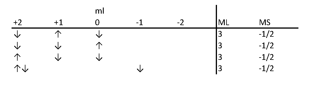
The method of using a table to count possible "microstates" has been developed so long ago and honed by so many scientists and educators that it is hard to accredit a single person. Let's take the electronic configuration of d3 as an example. In the Slater's table, each cell contains the number of ways to assign the three electrons quantum numbers according to the MS and ML values. These assignments follow Pauli's exclusion law. The figure below shows an example to find out how many ways to assign quantum numbers to d3 electrons when ML = 3 and MS = -1/2.

		MS
		-3/2	-1/2	1/2	3/2
ML	5	0	1	1	0
	4	0	2	2	0
	3	1	4	4	1
	2	1	6	6	1
	1	2	8	8	2
	0	2	8	8	2
	-1	2	8	8	2
	-2	1	6	6	1
	-3	1	4	4	1
	-4	0	2	2	0
	-5	0	1	1	0

Now we start to subtract term symbols from this table. First there is a 2H state. And now it is subtracted from the table.

		MS
		-3/2	-1/2	1/2	3/2
ML	5	0	0	0	0
	4	0	1	1	0
	3	1	3	3	1
	2	1	5	5	1
	1	2	7	7	2
	0	2	7	7	2
	-1	2	7	7	2
	-2	1	5	5	1
	-3	1	3	3	1
	-4	0	1	1	0
	-5	0	0	0	0

And now is a 4F state. After being subtracted by 4F, the table becomes

		MS
		-3/2	-1/2	1/2	3/2
ML	5	0	0	0	0
	4	0	1	1	0
	3	0	2	2	0
	2	0	4	4	0
	1	1	6	6	1
	0	1	6	6	1
	-1	1	6	6	1
	-2	0	4	4	0
	-3	0	2	2	0
	-4	0	1	1	0
	-5	0	0	0	0

And now 2G.

		MS
		-3/2	-1/2	1/2	3/2
ML	5	0	0	0	0
	4	0	0	0	0
	3	0	1	1	0
	2	0	3	3	0
	1	1	5	5	1
	0	1	5	5	1
	-1	1	5	5	1
	-2	0	3	3	0
	-3	0	1	1	0
	-4	0	0	0	0
	-5	0	0	0	0

Now 2F.

		MS
		-3/2	-1/2	1/2	3/2
ML	5	0	0	0	0
	4	0	0	0	0
	3	0	0	0	0
	2	0	2	2	0
	1	1	4	4	1
	0	1	4	4	1
	-1	1	4	4	1
	-2	0	2	2	0
	-3	0	0	0	0
	-4	0	0	0	0
	-5	0	0	0	0

Here in the table are two 2D states.

		MS
		-3/2	-1/2	1/2	3/2
ML	5	0	0	0	0
	4	0	0	0	0
	3	0	0	0	0
	2	0	0	0	0
	1	1	2	2	1
	0	1	2	2	1
	-1	1	2	2	1
	-2	0	0	0	0
	-3	0	0	0	0
	-4	0	0	0	0
	-5	0	0	0	0

4P.

		MS
		-3/2	-1/2	1/2	3/2
ML	5	0	0	0	0
	4	0	0	0	0
	3	0	0	0	0
	2	0	0	0	0
	1	0	1	1	0
	0	0	1	1	0
	-1	0	1	1	0
	-2	0	0	0	0
	-3	0	0	0	0
	-4	0	0	0	0
	-5	0	0	0	0

And the final deducted state is 2P. So in total the possible states for a d3 configuration are 4F, 4P, 2H, 2G, 2F, 2D, 2D and 2P. Taken J into consideration, the possible states are:

4F24F34F44P04P14P22H922H1122G922G722F722F522D522D522D322D322P322P32(16)$$\begin{array}{}\text{(16)}& {}^4{F}_2{}^4{F}_3{}^4{F}_4{}^4{P}_0{}^4{P}_1{}^4{P}_2{}^2{H}_{\frac{9}{2}}{}^2{H}_{\frac{11}{2}}{}^2{G}_{\frac{9}{2}}{}^2{G}_{\frac{7}{2}}{}^2{F}_{\frac{7}{2}}{}^2{F}_{\frac{5}{2}}{}^2{D}_{\frac{5}{2}}{}^2{D}_{\frac{5}{2}}{}^2{D}_{\frac{3}{2}}{}^2{D}_{\frac{3}{2}}{}^2{P}_{\frac{3}{2}}{}^2{P}_{\frac{3}{2}}\end{array}$$

For lighter atoms before or among the first-row transition metals, this method works well.

Using group theory to determine term symbols

Another method is to use direct products in group theory to quickly work out possible term symbols for a certain electronic configuration. Basically, both electrons and holes are taken into consideration, which naturally results in the same term symbols for complementary configurations like p2 vs p4. Electrons are categorized by spin, therefore divided into two categories, α and β, as are holes: α stands for +1, and βstands for -1, or vice versa. Term symbols of different possible configurations within one category are given. The term symbols for the total electronic configuration are derived from direct products of term symbols for different categories of electrons. For the p3configuration, for example, the possible combinations of different categories are eα3, eβ3, eα2eβ and eαeβ2. The first two combinations were assigned the partial term of S.6 As eα2 and eβ were given an P symbol, the combination of them gives their direct product

P × P = S + [P] + D.

The direct product for eα and eβ2 is also

P × P = S + [P] + D.

Considering the degeneracy, eventually the term symbols for p3 configuration are 4S, 2D and 2P.

There is a specially modified version of this method for atoms with 2 unpaired electrons. The only step gives the direct product of the symmetries of the two orbitals. The degeneracy is still determined by Pauli's exclusion.

Determining the ground state

In general, states with a greater degeneracy have a lower energy. For one configuration, the level with the largest S, which has the largest spin degeneracy, has the lowest energy. If two levels have the same S value, then the one with the larger L (and also the larger orbital degeneracy) have the lower energy. If the electrons in the subshell are fewer than half-filled, the ground state should have the smallest value of J, otherwise the ground state has the greatest value of J.

Electronic transitions

Electrons of an atom may undergo certain transitions which may have strong or weak intensities. There are rules about which transitions should be strong and which should be weak. Usually an electronic transition is excited by heat or radiation. Electronic states can be interpreted by solutions of Schrödinger's equation. Those solutions have certain symmetries, which are a factor of whether transitions will be allowed or not. The transition may be triggered by an electric dipole momentum, a magnetic dipole momentum, and so on. These triggers are transition operators. The most common and usually most intense transitions occur in an electric dipolar field, so the selection rules are

1. ΔL = 0, ±1 except L = 0 ‡ L' = 0
2. ΔS = 0
3. ΔJ = 0; ±1 except J = 0 ‡ J' = 0

where a double dagger means not combinable. For jj coupling, only the third rule applies with an addition rule: Δj = 0; ±1.